Simulating a network

One central piece is to have a network of workers and firms over time. We then start by simulating such an object. The rest of homework will focus on adding wages to this model. As we know from the lectures, a central issue of the network will be the number of movers.

We are going to model the mobility between workers and firms. Given a transition matrix we can solve for a stationary distrubtion, and then construct our panel from there.

p <- list()
p$nk = 30  # firm types
p$nl = 10  # worker types

p$alpha_sd = 1
p$psi_sd   = 1

# let's draw some FE
p$psi   = with(p,qnorm(1:nk/(nk+1)) * psi_sd)
p$alpha = with(p,qnorm(1:nl/(nl+1)) * alpha_sd)

# let's assume moving PR is fixed
p$lambda = 0.05

p$csort = 0.5 # sorting effect
p$cnetw = 0.2 # network effect
p$csig  = 0.5 # 

# lets create type specific transition matrices
# we are going to use joint normal centered on different values
# G[i,j,k] = Pr[worker i, at firm j, moves to firm k]
getG <- function(p){
  G = with(p,array(0,c(nl,nk,nk)))
  for (l in 1:p$nl) for (k in 1:p$nk) {
    # prob of moving is highest if dnorm(0)
    G[l,k,] = with(p,dnorm( psi - cnetw *psi[k] - csort * alpha[l],sd = csig ))
    # normalize to get transition matrix
    G[l,k,] = G[l,k,]/sum(G[l,k,])
  } 
  return(G)
}
G <- getG(p)


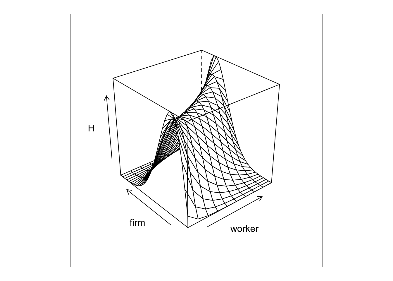
getH <- function(p,G){
  # we then solve for the stationary distribution over psis for each alpha value
  H = with(p,array(1/nk,c(nl,nk)))
  for (l in 1:p$nl) {
    M = G[l,,]
      for (i in 1:100) {
         H[l,] = t(G[l,,]) %*% H[l,]
      }
  }
  return(H)
}
H = getH(p,G)


Plot1=wireframe(G[1,,],aspect = c(1,1),xlab = "previous firm",ylab="next firm")
Plot2=wireframe(G[p$nl,,],aspect = c(1,1),xlab = "previous firm",ylab="next firm")
grid.arrange(Plot1, Plot2,nrow=1)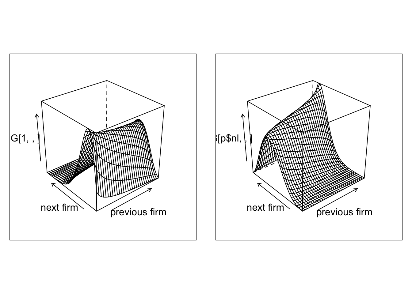

And we can plot the joint distribution of matches

wireframe(H,aspect = c(1,1),xlab = "worker",ylab="firm")

The next step is to simulate our network given our transitions rules.

p$nt = 5
p$ni = 130000

sim <- function(p,G,H){
  set.seed(1)

  # we simulate a panel
  network    = array(0,c(p$ni,p$nt))
  spellcount = array(0,c(p$ni,p$nt))
  A = rep(0,p$ni)
  
  for (i in 1:p$ni) {
    # we draw the worker type
    l = sample.int(p$nl,1)
    A[i]=l
    # at time 1, we draw from H
    network[i,1] = sample.int(p$nk,1,prob = H[l,])
    for (t in 2:p$nt) {
      if (runif(1)<p$lambda) {
        network[i,t] = sample.int(p$nk,1,prob = G[l,network[i,t-1],])
        spellcount[i,t] = spellcount[i,t-1] +1
      } else {
        network[i,t]    = network[i,t-1]
        spellcount[i,t] = spellcount[i,t-1]
      }
    }
  }
  
  data  = data.table(melt(network,c('i','t')))
  data2 = data.table(melt(spellcount,c('i','t')))
  setnames(data,"value","k")
  data[,spell := data2$value]
  data[,l := A[i],i]
  data[,alpha := p$alpha[l],l]
  data[,psi := p$psi[k],k]
}

data <- sim(p,G,H)

The final step is a to assign identities to the firm. We are going to do this is a relatively simple way, by simply randomly assigning firm ids to spells.

addSpells <- function(p,dat){
  firm_size = 10
  f_class_count = p$ni/(firm_size*p$nk*p$nt)
  
  dspell <- dat[,list(len=.N),list(i,spell,k)]
  dspell[,fid := sample( 1: pmax(1,sum(len)/f_class_count )   ,.N,replace=TRUE) , k]
  dspell[,fid := .GRP, list(k,fid)]
  
  setkey(dat,i,spell)
  setkey(dspell,i,spell)
  
  dat[, fid:= dspell[dat,fid]]
}

addSpells(p,data)  # adds by reference to the same data.table object (no copy needed)

Question 1 We are going to do some R-golfing (see wikipedia). I want you to use a one line code to evaluate the following 2 quantities:

• mean firm size, in the crossection, expect something like 15.
• mean number of movers per firm in total in our panel (a worker that moved from firm i to j is counted as mover in firm i as well as in firm j).

## [1] 17.36807

## [1] 28

## [1] 3.468003

## [1] 62

To evaluate the number of strokes that you needed to use run the following on your line of code: nchar("YOUR_CODE_IN_QUOTES_LIKE_THIS"). My scores for the previous two are 28 and 62.

Simulating AKM wages

We start with just AKM wages, which is log additive with some noise.

p$w_sigma = 0.8
addWage <- function(p,data){
  data[, lw := alpha + psi + p$w_sigma * rnorm(.N) ]
}
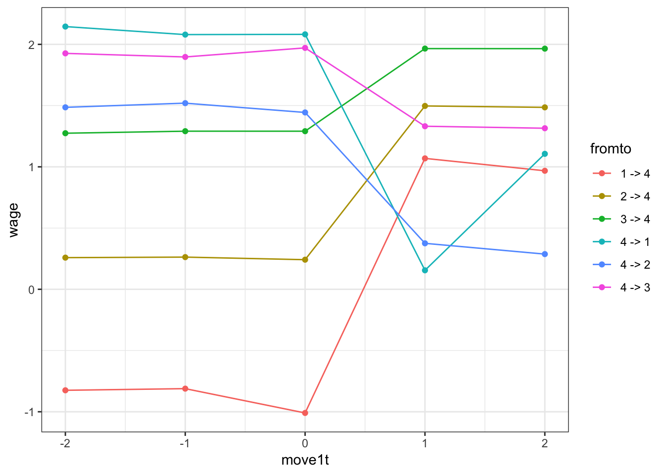
addWage(p,data)

Question 2 Before we finish with the simulation code, use this generated data to create the event study plot from Card-Heining-Kline:

1. Compute the mean wage within firm
2. group firms into quartiles
3. select workers around a move (2 periods pre, 2 periods post)
4. compute wages before/after the move for each transitions (from each quartile to each quartile)
5. plot the lines associated with each transition

Calibrating the parameters

Question 3 Pick the parameters psi_sd,alpha_sd,csort, csig and w_sigma to roughly match the decomposition in equation (6) of Card-Heining-Kline (note that they often report numbers in standard deviations, not in variances). psi_sd, alpha_sd, w_sigma can be directly calibrated from CHK. On the other hand, csort and csig needs to be calibrated to match the numbers in CHK after AKM estimation. If AKM estimation on psi and alpha is too slow, use the true psi and alpha and get residuals directly. For this last part, however, we first need to confront the question of how to actually estimate this AKM model!

Extracting the connected set

Because we are not going to deal with extremely large data-sets, we can use off the shelf algorithms to extract the connected set. There are two approaches:

1. Use the function conComp from the package ggm to extract the connected set from our data. To do so you will need to construct first an adjacency matrix between the firms. An adjacency matrix is a (number of fid,number of fid) square matrix. Element \((i,j)=1\) if a worker ever moved from \(i\) to \(j\), else \((i,j)=0\). Here is how I would proceed to construct the adjacency matrix:
   1. Append the lagged firm id as a new column in your data data[ ,fid.l1 := data[J(i,t-1),fid]], for which you need to first run setkey(data,i,t)
   2. Extract all moves from this data set jdata = data[fid.l1!=fid] and only keep unique pairs
   3. Then create a column value:=1 and cast this new data to an array using the acast command with fill=0
2. Use the function compfactor from package lfe. I prefer this approach because much faster.

Question 4 Use the previous procedure, extract the connected set, drop firms not in the set (I expect that all firms will be in the set).

adjMat <- function(data){
  setkey(data,i,t)
  data[ ,fid.l1 := data[J(i,t-1),fid]]
  data <- data[complete.cases(data)]
  nfirms = data[,max(fid)]
  jdata = data[fid.l1!=fid][,list(fid,fid.l1)]
  jdata = unique(jdata)
  setkey(jdata,fid,fid.l1)
  # jdata holds the indices where a sparse matrix should be 1.
  amat = Matrix::sparseMatrix(i=jdata[,c(fid,fid.l1)],j=jdata[,c(fid.l1,fid)],dims=c(nfirms,nfirms))
 amat
}

# amat = adjMat(data)
# g = graph.adjacency(as.matrix(amat))  # says it supports Matrix::sparsematrix, but doesn't...
# # plot(g)  # takes forever, shows unconnected firms
# clu = components(g)
# connected = groups(clu)
# # keep all in largest connected set
# keep = connected$`1`
# data = data[fid %in% keep]

# or, using lfe
concomp <- function(data){
  setkey(data,i,t)
  data[ ,fid.l1 := data[J(i,t-1),fid]]
  data <- data[complete.cases(data)]
  cf = lfe::compfactor(list(f1=data[,factor(fid)],f2=data[,factor(fid.l1)]))
  fr = data.frame(f1=data[,factor(fid)],f2=data[,factor(fid.l1)],cf)
  data = data[fr$cf==1]
  return(data)
}

data <- concomp(data)

Estimating worker and firms FE

Estimating this model is non-trivial. Traditional approaches like a within-transformation is not sufficient here, as we have two fixed effects to estimate. Guimareas and Portugal propose a ZigZag estimator in the Stata Journal. Simen Gaure proposes an almost equivalent approach and develops the lfe package for R. The idea in both approaches starts with the formulation

\[ \mathbf{Y} = \mathbf{Z}\beta + \mathbf{D}\alpha + \epsilon \]

where \(\mathbf{Z}\) is \((N,k)\), and \(\mathbf{D}\) is a \((N,G_1)\) matrix of dummy variables: element \((i,j)\) of \(\mathbf{D}\) is \(1\) if \(i\) is associated to \(j\).

Both papers show the recursive relationship

\[ \left[ \begin{array}{c} \beta &=& (\mathbf{Z}'\mathbf{Z})^{-1} \mathbf{Z}'(\mathbf{Y}-\mathbf{D}\alpha) \\ \alpha &=& (\mathbf{D}'\mathbf{D})^{-1} \mathbf{D}'(\mathbf{Y}-\mathbf{Z}\beta) \end{array} \right] \]

• line 2 is just data[,mean(resid(lm(y ~ z))),by=i]
• Dimensionality of \(\mathbf{D}\) becomes irrelevant.
• Same principle for more than 1 FE:

\[ \mathbf{Y} = \mathbf{Z}\beta + \mathbf{D}_1\alpha + \mathbf{D}_2\gamma + \epsilon \]

and recursive structure:

\[ \left[ \begin{array}{c} \beta &=& (\mathbf{Z}'\mathbf{Z})^{-1} \mathbf{Z}'(\mathbf{Y}-\mathbf{D}_1\alpha-\mathbf{D}_2\gamma) \\ \alpha &=& (\mathbf{D}_1'\mathbf{D}_1)^{-1} \mathbf{D}_1'(\mathbf{Y}-\mathbf{Z}\beta-\mathbf{D}_2\gamma) \\ \gamma &=& (\mathbf{D}_2'\mathbf{D}_2)^{-1} \mathbf{D}_2'(\mathbf{Y}-\mathbf{Z}\beta-\mathbf{D}_1\alpha) \end{array} \right] \]

• First, store a mod = data[,lm(y ~ z + D1 + D2)]
• line 2 is just data[,mean(resid(mod) + coef(mod)[3]*D2),by=i]
• line 3 is just data[,mean(resid(mod) + coef(mod)[2]*D1),by=j]

Guimaraes+Portugal do this in an iterative fashion until the difference in mean squared error (MSE) of successive estimates of line 0 becomes small.

Question 5 Write a function guimaraesPortugal that takes data and tol as an input and does the following steps:

1. add 2 columns alpha_hat=0 and psi_hat=0
2. get a list of mover ids
3. initiate delta=Inf
4. while delta>tol do
   1. run a lin reg of lw on psi_hat and alpha_hat
   2. store the coef
      1. if first iteration, override coef[2:3] <- 0
   3. get model residuals
   4. compute MSE for movers only
   5. compute new alpha_hat as mean of res + coefs[3]*alpha_hat by i, as above
   6. same for psi_hat
5. return the so updated data.table and check that the linear regression lm(lw ~ alpha_hat + psi_hat) has coefficients 1.00000 for both FEs.

## INFO [2018-11-08 10:00:07] iter=1, MSE=0.214216, delta(MSE)=Inf
## INFO [2018-11-08 10:00:14] iter=10, MSE=0.097778, delta(MSE)=0.000759
## INFO [2018-11-08 10:00:21] iter=20, MSE=0.093468, delta(MSE)=0.000246
## INFO [2018-11-08 10:00:29] iter=30, MSE=0.091924, delta(MSE)=0.000116
## INFO [2018-11-08 10:00:36] iter=40, MSE=0.091147, delta(MSE)=0.000067
## INFO [2018-11-08 10:00:43] iter=50, MSE=0.090681, delta(MSE)=0.000044
## INFO [2018-11-08 10:00:50] iter=60, MSE=0.090371, delta(MSE)=0.000030
## INFO [2018-11-08 10:00:57] iter=70, MSE=0.090155, delta(MSE)=0.000022
## INFO [2018-11-08 10:01:03] iter=80, MSE=0.089996, delta(MSE)=0.000016
## INFO [2018-11-08 10:01:11] iter=90, MSE=0.089877, delta(MSE)=0.000013
## INFO [2018-11-08 10:01:20] iter=100, MSE=0.089786, delta(MSE)=0.000010
## INFO [2018-11-08 10:01:27] iter=110, MSE=0.089714, delta(MSE)=0.000008
## INFO [2018-11-08 10:01:34] iter=120, MSE=0.089656, delta(MSE)=0.000006
## INFO [2018-11-08 10:01:41] iter=130, MSE=0.089610, delta(MSE)=0.000005
## INFO [2018-11-08 10:01:49] iter=140, MSE=0.089572, delta(MSE)=0.000004
## INFO [2018-11-08 10:01:57] iter=150, MSE=0.089541, delta(MSE)=0.000004
## INFO [2018-11-08 10:02:05] iter=160, MSE=0.089515, delta(MSE)=0.000003
## INFO [2018-11-08 10:02:12] iter=170, MSE=0.089493, delta(MSE)=0.000003
## INFO [2018-11-08 10:02:19] iter=180, MSE=0.089475, delta(MSE)=0.000002
## INFO [2018-11-08 10:02:26] iter=190, MSE=0.089459, delta(MSE)=0.000002

## 
## Call:
## lm(formula = lw ~ alpha_hat + psi_hat, data = data)
## 
## Residuals:
##      Min       1Q   Median       3Q      Max 
## -1.70312 -0.21353 -0.00044  0.21438  1.53969 
## 
## Coefficients:
##              Estimate Std. Error t value Pr(>|t|)    
## (Intercept) 0.0002860  0.0004406   0.649    0.516    
## alpha_hat   1.0001969  0.0013660 732.223   <2e-16 ***
## psi_hat     1.0004850  0.0019395 515.842   <2e-16 ***
## ---
## Signif. codes:  0 '***' 0.001 '**' 0.01 '*' 0.05 '.' 0.1 ' ' 1
## 
## Residual standard error: 0.3175 on 519317 degrees of freedom
## Multiple R-squared:  0.5281, Adjusted R-squared:  0.5281 
## F-statistic: 2.905e+05 on 2 and 519317 DF,  p-value: < 2.2e-16

Note You can increase speed by focusing on movers only first to recover the psi.

Question 5 Now do the same thing but use the function felm from package lfe. Write function gaureAKM which takes data and p as inputs.

## INFO [2018-11-08 10:02:27] running gaureAKM with lambda=0.050000
## INFO [2018-11-08 10:02:41] done.

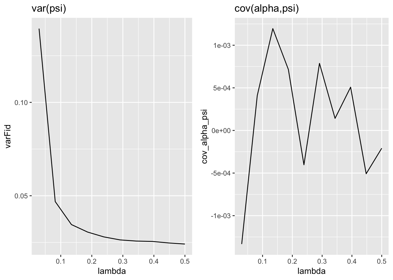
Alleviating the bias using Split Sample Jackknife

Pick a relatively short \(T\) together with a low \(\lambda\). Simulate one data-set. Next conduct the following procedure:

1. Estimate AKM on the full sample
2. Split your sample within firm, ie, within firm, split your movers in a balanced way between group 1 and group 2. Do the same for the individuals who don’t move. You can do that by assigning a random number to each worker within firm and then defining the group as being below or above the median.
3. Perform AKM on eash split-sample
4. Form average estimates of each parameter by just averaging over the subpanels: \(\overline{\theta}_{1/2} = 0.5 \hat{\theta}_{1} + 0.5 \hat{\theta}_{2}\)
5. Compute biased-corrected estimates for variance of firm-effects and covariances between worker and firm effects using the Split Panel Jackknife by Dhaene and Jochmans: use \(2 \hat{\theta} - \overline{\theta}_{1/2}\)

The theta in the bias correction formula is on var(psi), not psi itself.

Question 7 Report the true values, the non biased corrected and the bias corrected.