Using the GPU to do Value Function Iteration
Florian Oswald
This tutorial is inspired Tim Holy's introduction to GPU for Julia. Here we implement a custom Kernel to compute a simple value function iteration (VFI) algorithm. That part of the tutorial is based on Fernandez-Villaverde and Zarruk's parallel computing survey for Economists. For a good introduction to the computational side of value function iteration, I recommend the corresponding QuantEcon tutorial.
Setup
We create a function to build our parameter vector.
function param(;nx=1500,ne=15,T=10)
    p = (
        nx         = nx,
        xmax       = 4.0,
        xmin       = 0.1,
        ne         = ne,
        sigma_eps  = 0.02058,
        lambda_eps = 0.99,
        m          = 1.5,
        sigma      = 2,
        beta       = 0.97,
        T          = 10,
        r          = 0.07,
        w          = 5,
        xgrid      = zeros(Float32,nx),
        egrid      = zeros(Float32,ne),
        P          = zeros(Float32,ne,ne))


    # populate transition matrix

    # Grid for capital (x)
    p.xgrid[:] = collect(range(p.xmin,stop=p.xmax,length=p.nx));

    # Grid for productivity (e) with Tauchen (1986)
    sigma_y = sqrt((p.sigma_eps^2) / (1 - (p.lambda_eps^2)));
    estep = 2*sigma_y*p.m / (p.ne-1);
    for i = 1:p.ne
        p.egrid[i] = (-p.m*sqrt((p.sigma_eps^2) / (1 - (p.lambda_eps^2))) + (i-1)*estep);
    end

    # Transition probability matrix (P) Tauchen (1986)
    mm = p.egrid[2] - p.egrid[1];
    for j = 1:p.ne
        for k = 1:p.ne
            if(k == 1)
                p.P[j, k] = cdf(Normal(), (p.egrid[k] - p.lambda_eps*p.egrid[j] + (mm/2))/p.sigma_eps);
            elseif(k == ne)
                p.P[j, k] = 1 - cdf(Normal(), (p.egrid[k] - p.lambda_eps*p.egrid[j] - (mm/2))/p.sigma_eps);
            else
                p.P[j, k] = cdf(Normal(), (p.egrid[k] - p.lambda_eps*p.egrid[j] + (mm/2))/p.sigma_eps) - cdf(Normal(), (p.egrid[k] - p.lambda_eps*p.egrid[j] - (mm/2))/p.sigma_eps);
            end
        end
    end

    # exponential of egrid
    p.egrid[:] = exp.(p.egrid)
    return p
end
param (generic function with 1 method)
let's get an instance of it.
using Distributions
p = param()
Computing the value function at a single state
A state in our setup is a triple (ix,ie,age), i.e. a value of capital and endowment shock. Here is how we could do this:
function v(ix::Int,ie::Int,age::Int,Vnext::Matrix{Float64},p::NamedTuple)

    out = typemin(eltype(Vnext))
    ixpopt = 0 # optimal policy
    expected = 0.0
    utility = out
    for jx in 1:p.nx
        if age < p.T
            for je in 1:p.ne
                expected += p.P[ie,je] * Vnext[jx,je]
            end
        end
        cons = (1+p.r)*p.xgrid[ix] + p.egrid[ie]*p.w - p.xgrid[jx]
        utility = (cons^(1-p.sigma))/(1-p.sigma) + p.beta * expected
        if cons <= 0
            utility = typemin(eltype(Vnext))
        end
        if utility >= out
            out = utility
            ixpopt = jx
        end
    end
    return out
end
v (generic function with 1 method)
and finally, a function that cycles over age and each state
function cpu_lifecycle(p::NamedTuple)
    V = zeros(p.nx,p.ne,p.T)
    Vnext = zeros(p.nx,p.ne)
    for age in p.T:-1:1
        for ix in 1:p.nx
            for ie in 1:p.ne
                value = v(ix,ie,age,Vnext,p)
                V[ix,ie,age] = value
            end
        end
        Vnext[:,:] = V[:,:,age]
    end
    println("first three shock states at age 1: $(V[1,1:3,1])")
    return V
end

vcpu = cpu_lifecycle(p);
first three shock states at age 1: [-2.12087, -2.08143, -2.02839]
Let's make a plot of the resulting value function:
using Plots
CList = reshape( range(colorant"yellow", stop=colorant"red",length=p.ne), 1, p.ne );
p1 = plot(p.xgrid,vcpu[:,:,1],
    linecolor=CList,
    title="period 1",
    leg=false,label=["e$i" for i in 1:p.ne],xlabel="x",ylabel="v(x)")
p2 = plot(p.xgrid,vcpu[:,:,p.T-1],
    linecolor=CList,
    title="period T-1",
    leg=:bottomright,label=["e$i" for i in 1:p.ne],xlabel="x",ylabel="v(x)")
plot(p1,p2,layout=2, link=:y)

Parallelizing on the CPU
Multicore
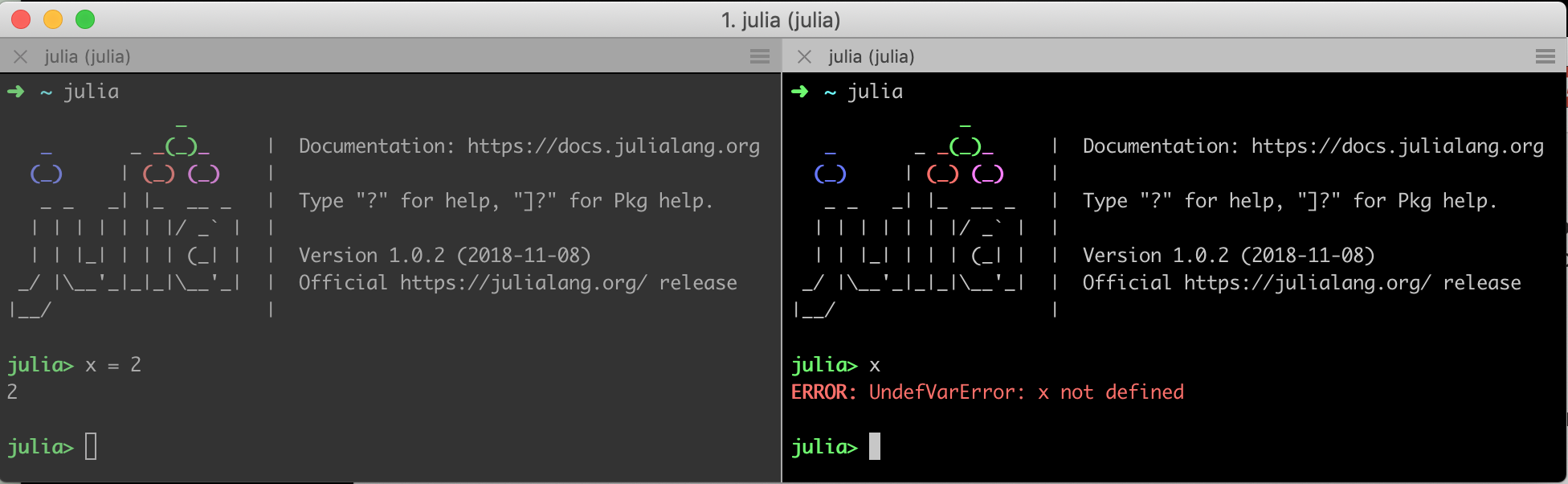
Multicore computation distributes the work across multiple worker nodes. A slight complication with the distributed model is that the worker processes use separate memory - even if they reside in the same machine! I find it easiest to imagine that you start several separate julia processes in your terminal, each in their own tab. Clearly, creating x=2 in the first processes doesn't make the object x available in the other processes. This is true for data (like x), as it is for code. Any function you want to call on one of the worker processes must be defined on that process. Again visualize the separate terminal windows, and imagine defining function f() on process 1. Calling f() on process 2 will return an error. This is illustrated here:
The Distributed package provides functionality to efficiently connect those separate processes, and the SharedArrays package gives us an Array type which may be shared by several processes. The function workers() shows the ids of the currently active workers. By default, this is just a single worker, which we also often call the master node:
using SharedArrays
using Distributed

workers()
addprocs(5)  # add 5 workers
5-element Array{Int64,1}:
 2
 3
 4
 5
 6
Let's define a function that distributes the computation of each state (ix,ie) over our set of workers. the main thing to look out for is that we have to make the function v available on all workers. We could save it to a file script.jl, for example, and load julia with the command line option --load script.jl. Alternatively, we redefine it here, by prefix with the macro @everywhere:
@everywhere function v(ix::Int,ie::Int,age::Int,Vnext::Matrix{Float64},p::NamedTuple)

    out = typemin(eltype(Vnext))
    ixpopt = 0 # optimal policy
    expected = 0.0
    utility = out
    for jx in 1:p.nx
        if age < p.T
            for je in 1:p.ne
                expected += p.P[ie,je] * Vnext[jx,je]
            end
        end
        cons = (1+p.r)*p.xgrid[ix] + p.egrid[ie]*p.w - p.xgrid[jx]
        utility = (cons^(1-p.sigma))/(1-p.sigma) + p.beta * expected
        if cons <= 0
            utility = typemin(eltype(Vnext))
        end
        if utility >= out
            out = utility
            ixpopt = jx
        end
    end
    return out
end
Now that this is defined on all workers, we can move on to define the calling function on the master node. Notice that we have to use a SharedArray for the worker processes to save their results in - remember that by default they would not have access to a standard Array created on the master worker.
function cpu_lifecycle_multicore(p::NamedTuple)
    println("julia running with $(length(workers())) workers")
    V = zeros(p.nx,p.ne,p.T)
    Vnext = zeros(p.nx,p.ne)
    Vshared = SharedArray{Float64}(p.nx,p.ne)   # note!
    for age in p.T:-1:1
        @sync @distributed for i in 1:(p.nx*p.ne)   # distribute over a single index
            ix,ie = Tuple(CartesianIndices((p.nx,p.ne))[i])
            value = v(ix,ie,age,Vnext,p)
            Vshared[ix,ie] = value
        end
        V[:,:,age] = Vshared
        Vnext[:,:] = Vshared
    end
    println("first three shock states at age 1: $(V[1,1:3,1])")
    return V
end
cpu_lifecycle_multicore (generic function with 1 method)
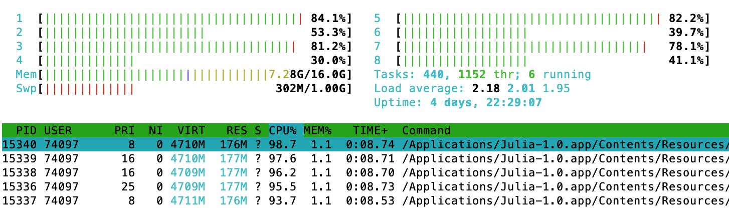
Important: Notice that the worker processes do not have to reside on the same machine, as in this example was indeed the case. The function addprocs is very powerful, so check out ?addprocs. In particular, one can simply supply a list of machine identifiers (like for instance IP addresses) to the function. It is interesting to look at the output of htop (or Activity Monitor on OSX) and see several different julia processes doing work, when we call this function:
Multithread
Related to this is the multithread model of parallelization. The good thing here is that we operate in shared memory, i.e. we don't have worry about moving data or code around - there is just a single julia session running in your imaginary terminal from above. What is happening, however, is that julia operates several threads through our CPU, whenever we tell it to do so with the macro Threads.@threads. One needs to be very careful to write such code in thread-safe way, that is, no 2 threads should want to write to the same array index, for example. Similarly to having to add workers via addprocs as above, here we have to start julia with multiple threads. You can achieve that by starting julia via
JULIA_NUM_THREADS=4 julia
Here is our lifecycle problem with a threaded loop:
function cpu_lifecycle_thread(p::NamedTuple)
    println("julia running with $(Threads.nthreads()) threads")
    V = zeros(p.nx,p.ne,p.T)
    Vnext = zeros(p.nx,p.ne)
    for age in p.T:-1:1
        Threads.@threads for i in 1:(p.nx*p.ne)
            ix,ie = Tuple(CartesianIndices((p.nx,p.ne))[i])
            value = v(ix,ie,age,Vnext,p)
            V[ix,ie,age] = value
        end
        Vnext[:,:] = V[:,:,age]
    end
    println("first three shock states at age 1: $(V[1,1:3,1])")
    return V
end
cpu_lifecycle_thread (generic function with 1 method)
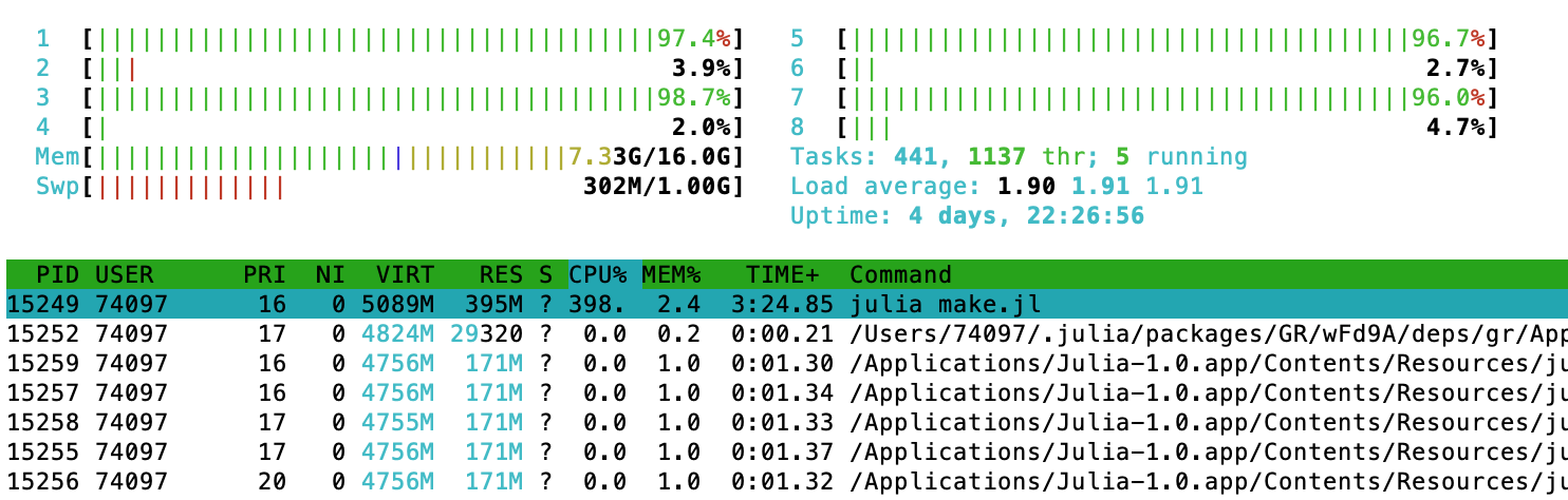
and, again, it's instructive to look at the system monitor via htop or similar. Now we see that a single process (the process that builds this page, executing julia make.jl) runs at almost 400% CPU utilization. The other worker processes are idle.
CPU Benchmarks
Before worrying about speed, we always want to verify that our computations are accurate. Taking the content of vcpu as the truth, let's see how close we get with the threaded computation:
vthread = cpu_lifecycle_thread(p);
julia running with 4 threads
first three shock states at age 1: [-2.12087, -2.08143, -2.02839]
using Test
@test vthread ≈ vcpu
Test Passed
You can see that I used the symbol ≈ here, which means approximately equal. In the julia REPL you obtain this by typing \approx<TAB>. Now let's worry about speed. Benchmarking incurs machine noise. This is very similar to any statistical sampling proceedure. Consider those timings obtained from a naive timing, for example:
@time cpu_lifecycle(p);
first three shock states at age 1: [-2.12087, -2.08143, -2.02839]
  7.887026 seconds (73 allocations: 3.797 MiB)
@time cpu_lifecycle(p);
first three shock states at age 1: [-2.12087, -2.08143, -2.02839]
  7.866052 seconds (73 allocations: 3.797 MiB)
@time cpu_lifecycle(p);
first three shock states at age 1: [-2.12087, -2.08143, -2.02839]
  7.868888 seconds (73 allocations: 3.797 MiB)
You can see that they all differ. If we were benchmarking a function that runs quickly, we could use the BenchmarkTools package. It basically runs the benchmark function many times and reports summary statistics. For long-running functions like ours, it will only take one sample, so the standard @time will do for us.
@time cpu_lifecycle(p);
first three shock states at age 1: [-2.12087, -2.08143, -2.02839]
  7.858191 seconds (73 allocations: 3.797 MiB)
@time cpu_lifecycle_thread(p);
julia running with 4 threads
first three shock states at age 1: [-2.12087, -2.08143, -2.02839]
  2.126724 seconds (377 allocations: 3.803 MiB, 0.19% gc time)
@time cpu_lifecycle_multicore(p)
julia running with 5 workers
first three shock states at age 1: [-2.12087, -2.08143, -2.02839]
julia running with 5 workers
  2.521773 seconds (10.19 k allocations: 2.753 MiB)
Process(`/home/floswald/apps/julia-1.0.0/bin/julia -Cnative -J/home/floswal
d/apps/julia-1.0.0/lib/julia/sys.so --compile=yes --depwarn=yes /home/flosw
ald/git/CuArrays.jl/tutorials/src/addprocs-vfi.jl`, ProcessExited(0))
Looking at those results its important to realise that we didn't cut the runtime by exactly the number of processes we ran - quite far from it, actually. It is very rare that our parallelization would achieve this so-called linear speedup. Overhead from communication between the various processes (threads or workers) is a crucial component of non-linear speedup. A simple rule of thumb is to avoid data movement between processes as much as possible; unfortunately optimizing parallel solutions beyond that simple rule requires knowledge that goes beyond this tutorial (and its author's knowledge as well).
Parallelizing on the GPU
using CuArrays
using CUDAnative

function v_gpu!(V,nx,ne,T,xgrid,egrid,r,w,sigma,beta,P,age)

    badval = -1_000_000.0f0
    vtmp = badval  # intiate V at lowest value
    ixpopt = 0 # optimal policy
    expected = 0.0f0
    utility = badval

    # strided loop
    index = (blockIdx().x - 1) * blockDim().x + threadIdx().x
    stride = blockDim().x * gridDim().x

    for i = index:stride:(nx*ne)

        ix = ceil(Int,i/ne)
        ie = ceil(Int,mod(i-0.05,ne))
        # @cuprintf("threadIdx %ld, blockDim %ld,ix %ld, ie %ld\n", index, stride,ix,ie)
        j = ix + nx*(ie-1 + ne*(age-1))
        vtmp = badval  # intiate V at lowest value
        for jx in 1:nx
            if age < T
                for je in 1:ne
                    expected = expected + P[ie,je] * V[jx + nx*(je-1 + ne*(age))]
                end
            end
            cons = convert(Float32,(1+r)*xgrid[ix] + egrid[ie]*w - xgrid[jx])
            utility = CUDAnative.pow(cons,convert(Float32,(1-sigma)))/(1-sigma) + beta * expected
            if cons <= 0
                utility = badval
            end
            if utility >= vtmp
                vtmp = utility
            end
        end
        V[j] = vtmp

    end
    return nothing
end

V_d = CuArray(zeros(Float32,p.nx,p.ne,p.T));
xgrid_d = CuArray(p.xgrid);
egrid_d = CuArray(p.egrid);
P_d = CuArray(p.P);

block_size = 256

@cuda threads=ceil(Int,(p.nx*p.ne)/block_size) blocks=block_size v_gpu!(V_d,p.nx,p.ne,p.T,xgrid_d,egrid_d,p.r,p.w,p.sigma,p.beta,P_d,p.T)

function bench_v_gpu!(V_d,nx,ne,T,xgrid_d,egrid_d,r,w,sigma,beta,P_d,age,block_size)
    CuArrays.@sync begin
        @cuda threads=ceil(Int,(nx*ne)/block_size) blocks=block_size v_gpu!(V_d,nx,ne,T,xgrid_d,egrid_d,r,w,sigma,beta,P_d,age)
    end
end

bench_v_gpu!(V_d,p.nx,p.ne,p.T,xgrid_d,egrid_d,p.r,p.w,p.sigma,p.beta,P_d,2,block_size);
using BenchmarkTools
@btime bench_v_gpu!(V_d,p.nx,p.ne,p.T,xgrid_d,egrid_d,p.r,p.w,p.sigma,p.beta,P_d,2,block_size)
143.363 ms (42 allocations: 1.47 KiB)
# using CUDAdrv
# CUDAdrv.@profile bench_v_gpu!(V_d,p.nx,p.ne,p.T,xgrid_d,egrid_d,p.r,p.w,p.sigma,p.beta,P_d,2,block_size)
# exit()
over the lifecycle
function gpu_lifecycle(p::NamedTuple)
    V_d = CuArray(zeros(Float32,p.nx,p.ne,p.T));
    xgrid_d = CuArray(p.xgrid);
    egrid_d = CuArray(p.egrid);
    P_d = CuArray(p.P);

    block_size = 256

    for it in p.T:-1:1
        @cuda threads=ceil(Int,(p.nx*p.ne)/block_size) blocks=block_size v_gpu!(V_d,p.nx,p.ne,p.T,xgrid_d,egrid_d,p.r,p.w,p.sigma,p.beta,P_d,it)
    end
    out = Array(V_d)  # download data from GPU
    println("first three shock states at age 1: $(out[1,1:3,1])")
    return out
end

gpu_lifecycle(p);  # compile
first three shock states at age 1: Float32[-2.12087, -2.08143, -2.02839]
@btime gpu_lifecycle(p);
first three shock states at age 1: Float32[-2.12087, -2.08143, -2.02839]
first three shock states at age 1: Float32[-2.12087, -2.08143, -2.02839]
first three shock states at age 1: Float32[-2.12087, -2.08143, -2.02839]
first three shock states at age 1: Float32[-2.12087, -2.08143, -2.02839]
first three shock states at age 1: Float32[-2.12087, -2.08143, -2.02839]
first three shock states at age 1: Float32[-2.12087, -2.08143, -2.02839]
first three shock states at age 1: Float32[-2.12087, -2.08143, -2.02839]
first three shock states at age 1: Float32[-2.12087, -2.08143, -2.02839]
  1.817 s (481 allocations: 2.60 MiB)
@btime cpu_lifecycle(p);
first three shock states at age 1: [-2.12087, -2.08143, -2.02839]
first three shock states at age 1: [-2.12087, -2.08143, -2.02839]
first three shock states at age 1: [-2.12087, -2.08143, -2.02839]
first three shock states at age 1: [-2.12087, -2.08143, -2.02839]
  7.921 s (113 allocations: 3.61 MiB)
how costly is it to create the CuArrays? Let's create them beforehand.
function gpu_lifecycle2(p::NamedTuple,V_d,xgrid_d,egrid_d,P_d)

    block_size = 256

    for it in p.T:-1:1
        @cuda threads=ceil(Int,(p.nx*p.ne)/block_size) blocks=block_size v_gpu!(V_d,p.nx,p.ne,p.T,xgrid_d,egrid_d,p.r,p.w,p.sigma,p.beta,P_d,it)
    end
    out = Array(V_d)  # download data from GPU
    println("first three shock states at age 1: $(out[1,1:3,1])")
    return out
end

V_d = CuArray(zeros(Float32,p.nx,p.ne,p.T));
xgrid_d = CuArray(p.xgrid);
egrid_d = CuArray(p.egrid);
P_d = CuArray(p.P);

gpu_lifecycle2(p,V_d,xgrid_d,egrid_d,P_d);
first three shock states at age 1: Float32[-2.12087, -2.08143, -2.02839]
@btime gpu_lifecycle2(p,V_d,xgrid_d,egrid_d,P_d);
first three shock states at age 1: Float32[-2.12087, -2.08143, -2.02839]
first three shock states at age 1: Float32[-2.12087, -2.08143, -2.02839]
first three shock states at age 1: Float32[-2.12087, -2.08143, -2.02839]
first three shock states at age 1: Float32[-2.12087, -2.08143, -2.02839]
first three shock states at age 1: Float32[-2.12087, -2.08143, -2.02839]
first three shock states at age 1: Float32[-2.12087, -2.08143, -2.02839]
first three shock states at age 1: Float32[-2.12087, -2.08143, -2.02839]
first three shock states at age 1: Float32[-2.12087, -2.08143, -2.02839]
  1.805 s (419 allocations: 893.27 KiB)
@btime cpu_lifecycle(p);
first three shock states at age 1: [-2.12087, -2.08143, -2.02839]
first three shock states at age 1: [-2.12087, -2.08143, -2.02839]
first three shock states at age 1: [-2.12087, -2.08143, -2.02839]
first three shock states at age 1: [-2.12087, -2.08143, -2.02839]
  7.910 s (112 allocations: 3.61 MiB)
not overly costly.
# We could again benchmark this with `nvprof`
using CUDAdrv
CUDAdrv.@profile gpu_lifecycle(p);
==14101== NVPROF is profiling process 14101, command: julia test2.jl
==14101== Profiling application: julia test2.jl
==14101== Profiling result:
   Start  Duration            Grid Size      Block Size     Regs*    ...
14.9753s  70.178us                    -               -         -    ...
14.9754s  1.0240us                    -               -         -    ...
14.9754s     512ns                    -               -         -    ...
14.9754s     608ns                    -               -         -    ...
15.1679s  1.75753s            (256 1 1)        (88 1 1)       206    ...
16.9255s  69.122us                    -               -         -    ...

Regs: Number of registers used per CUDA thread. This number includes ...
Results depend on problem size?
For the current problem size, the GPU solution is about as fast as the multithreaded one with 4 threads. How does this vary with problem size?
psmall = param(nx=150,ne=5)
pbig   = param(nx=2000,ne=25,T=100)


@time cpu_lifecycle(psmall);
first three shock states at age 1: [-2.16987, -1.94911, -1.7484]
  0.016509 seconds (64 allocations: 320.609 KiB)
@time cpu_lifecycle(pbig);
first three shock states at age 1: [-2.12024, -2.10028, -2.07342]
 32.092092 seconds (122 allocations: 8.204 MiB, 0.01% gc time)
@time cpu_lifecycle_thread(psmall);
julia running with 4 threads
first three shock states at age 1: [-2.16987, -1.94911, -1.7484]
  0.007863 seconds (371 allocations: 326.969 KiB)
@time cpu_lifecycle_thread(pbig);
julia running with 4 threads
first three shock states at age 1: [-2.12024, -2.10028, -2.07342]
  8.500026 seconds (428 allocations: 8.210 MiB, 0.02% gc time)
@time gpu_lifecycle(psmall);
first three shock states at age 1: Float32[-2.16987, -1.94911, -1.7484]
  0.071450 seconds (502 allocations: 300.016 KiB)
@time gpu_lifecycle(pbig);
first three shock states at age 1: Float32[-2.12024, -2.10028, -2.07342]
  7.181435 seconds (605 allocations: 5.941 MiB, 0.03% gc time)
==16667== NVPROF is profiling process 16667, command: julia test.jl
WARNING: using CUDAdrv.CuArray in module Main conflicts with an existing identifier.
==16667== Profiling application: julia test.jl
==16667== Profiling result:
   Start  Duration            Grid Size      Block Size     Regs*  ...           Device
19.9770s  163.30us                    -               -         -  ...  GeForce GTX 105
19.9772s  1.2160us                    -               -         -  ...  GeForce GTX 105
19.9772s     544ns                    -               -         -  ...  GeForce GTX 105
19.9772s     736ns                    -               -         -  ...  GeForce GTX 105
20.1390s  123.01ms            (256 1 1)       (196 1 1)       182  ...  GeForce GTX 105
20.2621s  765.93ms            (256 1 1)       (196 1 1)       182  ...  GeForce GTX 105
21.0280s  766.03ms            (256 1 1)       (196 1 1)       182  ...  GeForce GTX 105
21.7940s  765.93ms            (256 1 1)       (196 1 1)       182  ...  GeForce GTX 105
22.5600s  765.92ms            (256 1 1)       (196 1 1)       182  ...  GeForce GTX 105
23.3259s  765.94ms            (256 1 1)       (196 1 1)       182  ...  GeForce GTX 105
24.0918s  765.78ms            (256 1 1)       (196 1 1)       182  ...  GeForce GTX 105
24.8576s  765.84ms            (256 1 1)       (196 1 1)       182  ...  GeForce GTX 105
25.6234s  765.91ms            (256 1 1)       (196 1 1)       182  ...  GeForce GTX 105
26.3893s  765.95ms            (256 1 1)       (196 1 1)       182  ...  GeForce GTX 105
27.1553s  153.96us                    -               -         -  ...  GeForce GTX 105