library(sf)Linking to GEOS 3.11.0, GDAL 3.5.3, PROJ 9.1.0; sf_use_s2() is TRUERSciencesPo Intro To Programming 2023
11 October, 2024
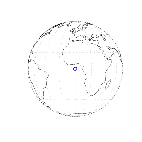
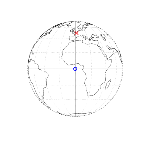
c(2.34,48.85) in WGS64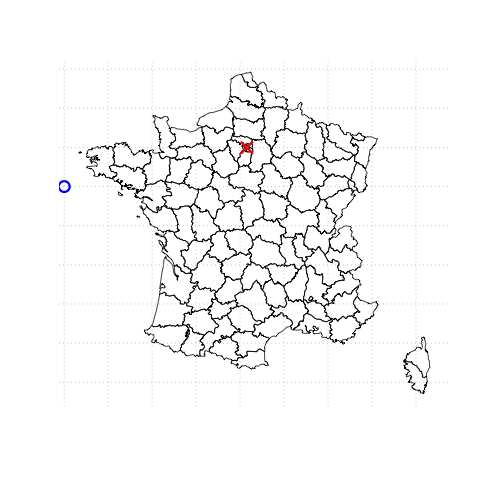
c(600256.4, 127726.4) in NTF Lambert North France
c(600256.4, 127726.4) in NTF Lambert North France
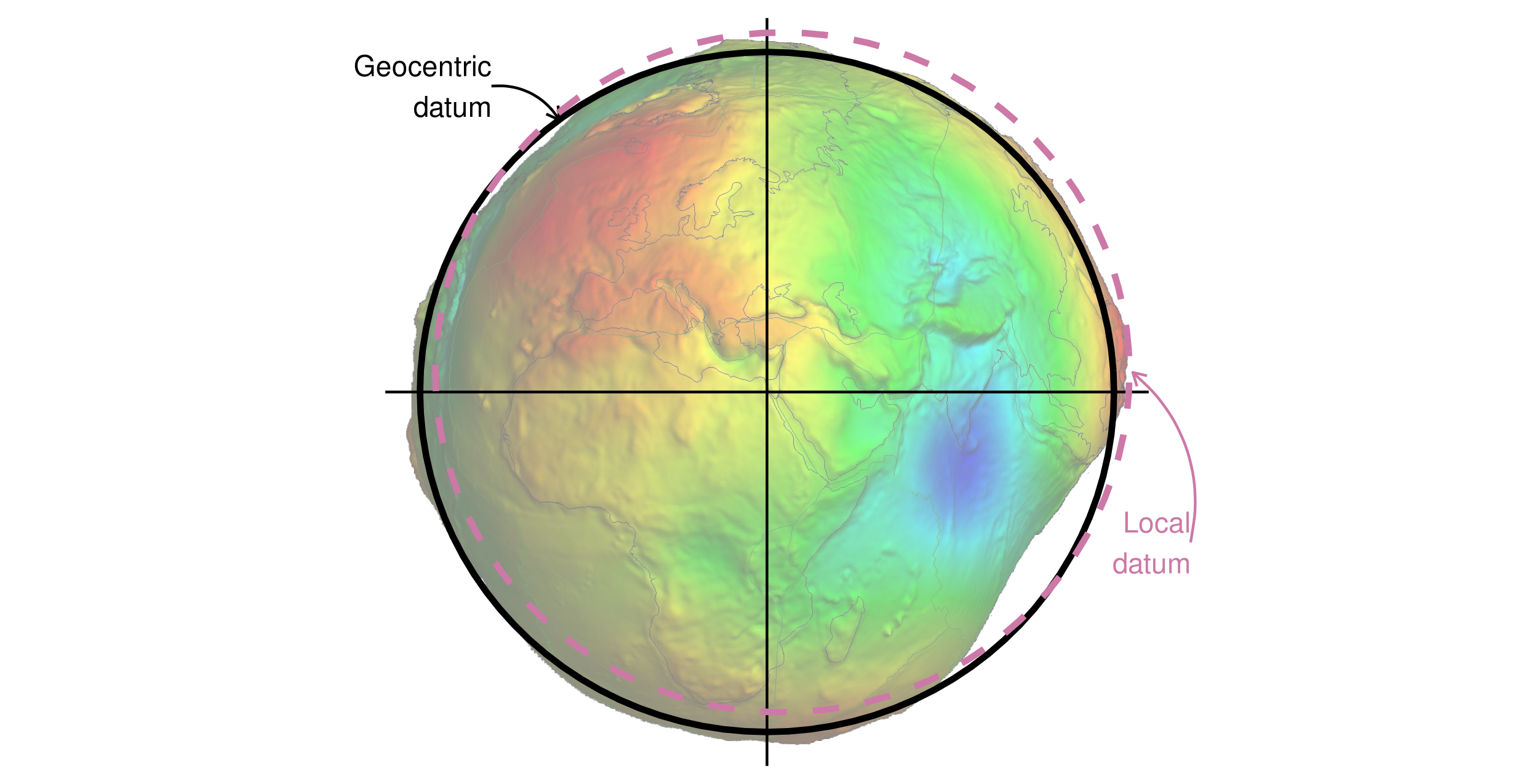
c(600256.4, 127726.4) actually mean?Figure from Geocomputation with R. Geocentric and local geodetic datums shown on top of a geoid (in false color and the vertical exaggeration by 10,000 scale factor). Image of the geoid is adapted from the work of Ince et al. (2019)
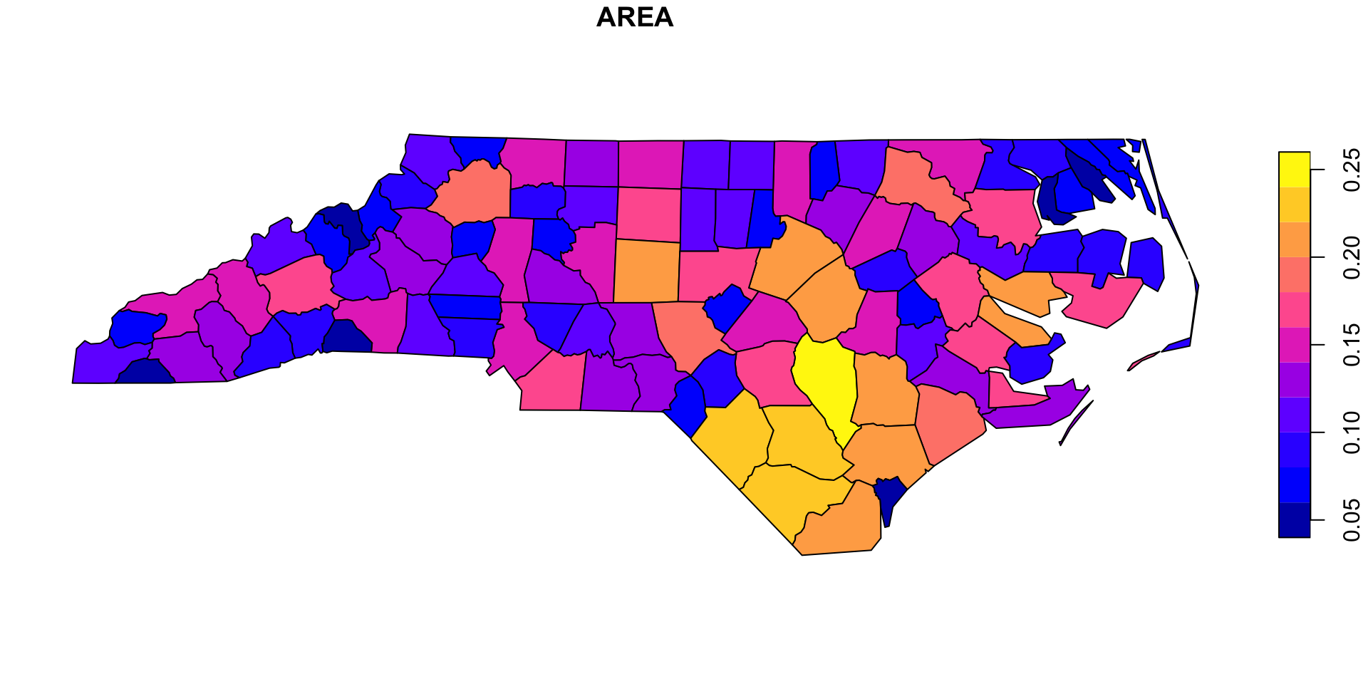
geometry column.data.frame.plot(nc[,"AREA"]) # plot feature "AREA" (i.e. column 1)ggplot2library(ggplot2)
ggplot(nc) + geom_sf(aes(fill = AREA)) +
scale_fill_viridis_c(name = "Area")ggplot(nc) + geom_sf(aes(fill = AREA)) +
scale_fill_viridis_c(name = "Area")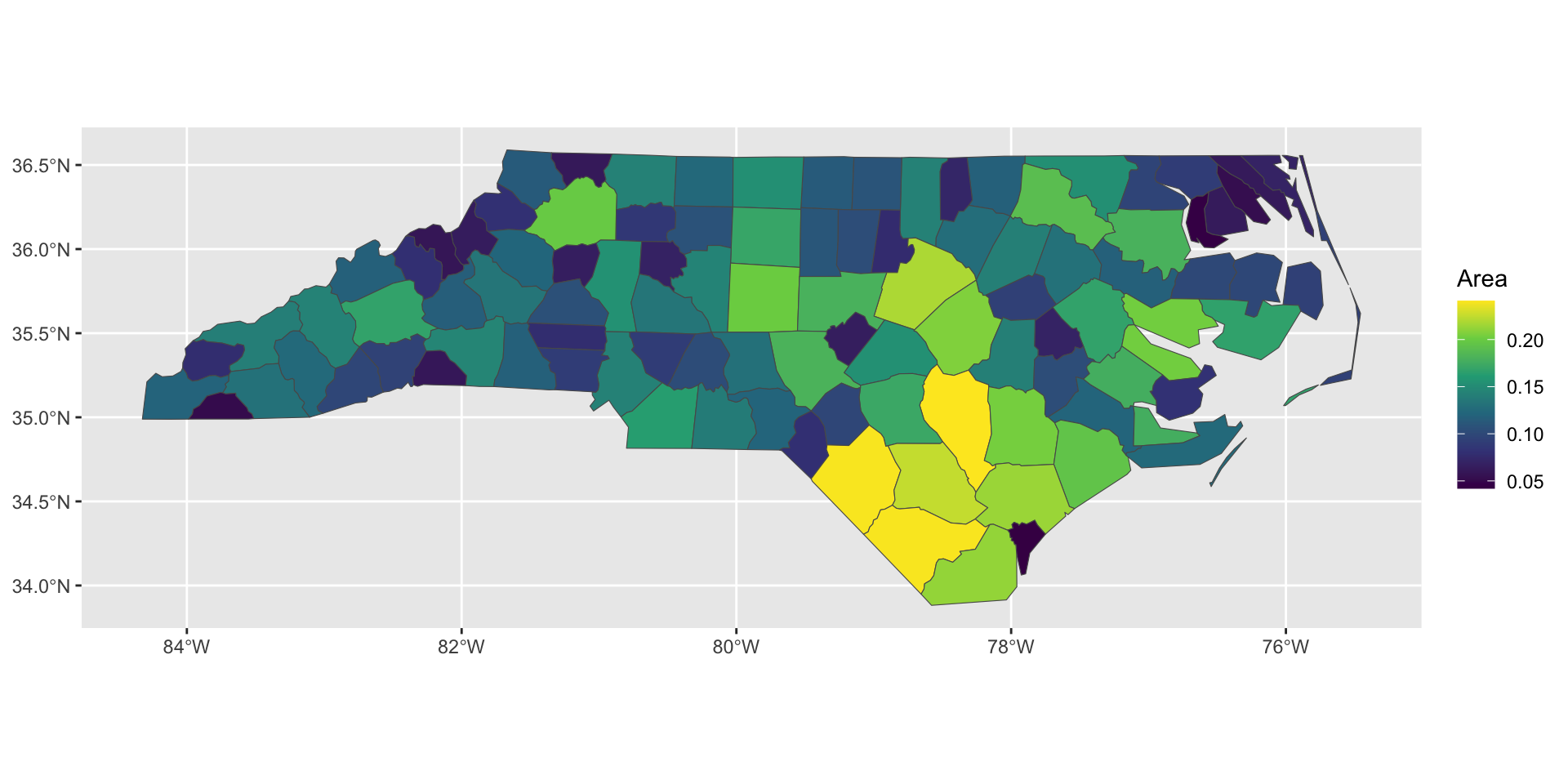
nc %>%
    st_transform("+proj=moll") %>%
    ggplot() + geom_sf(aes(fill = AREA)) +
        scale_fill_viridis_c(name = "Area") +
        ggtitle("Mollweide Projection")
# copied from https://github.com/uo-ec607/lectures
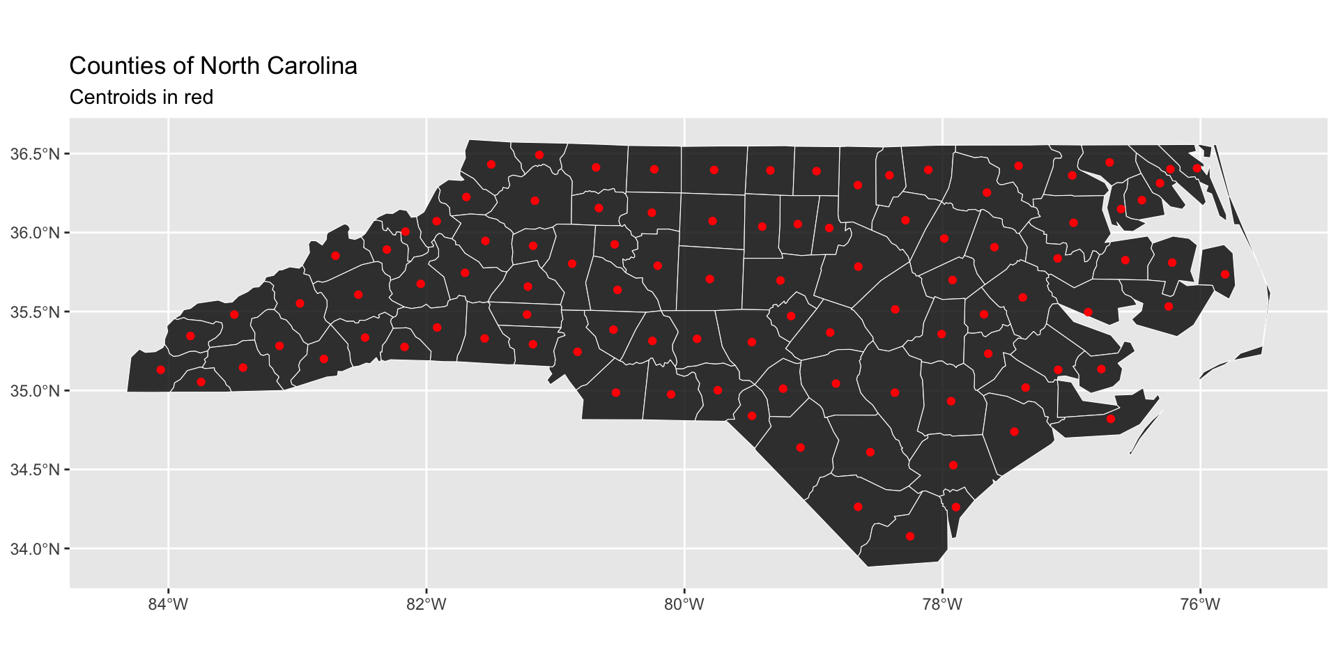
nc_centroid = st_centroid(nc)
ggplot(nc) +
geom_sf(fill = "black", alpha = 0.8, col = "white") +
geom_sf(data = nc_centroid, col = "red") + ## Notice how easy it is to combine different sf objects
labs(
title = "Counties of North Carolina",
subtitle = "Centroids in red"
)
Hint:
# start from here
p6 = ggplot(d5) + geom_sf()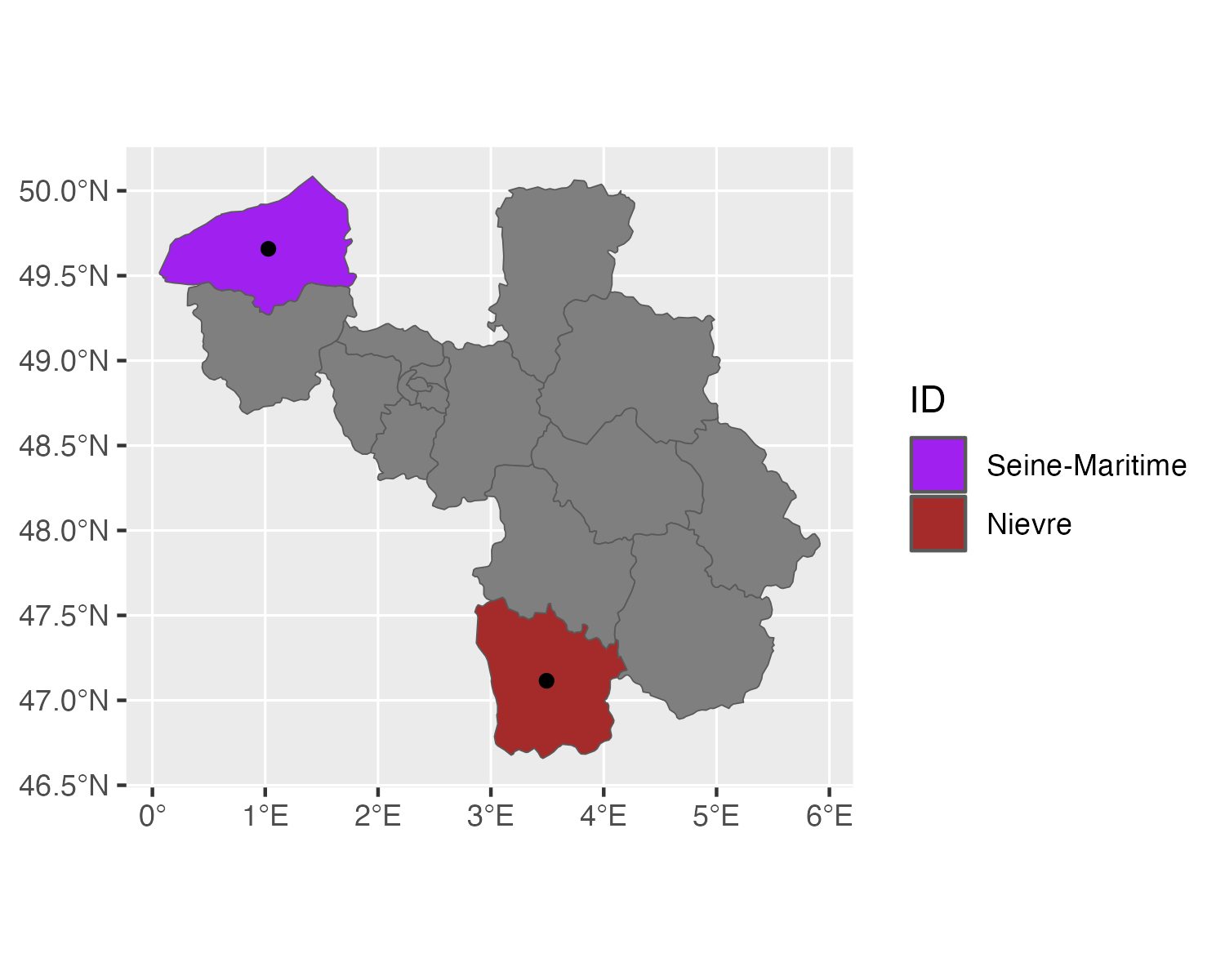
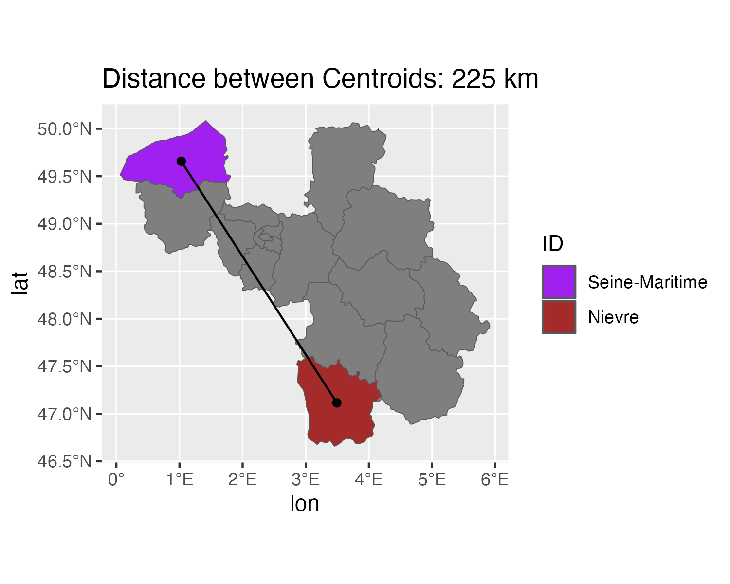
Desired Outputs
![]()