EM Benchmarks

Jul 6, 2019 7 min read

I am getting into estimating mixture models at the moment. In particular in the context of models of wage formation where unobserved heterogeneity stemming from both firm and worker side is often modeled with a mixture model. The main assumptions are that

Firms are classifiable into types $l \in \{1,\dots,L\}$, workers into $k \in \{1,\dots,K\}$
If Worker $i$ is of type $k$ and works for firm $l$ in a certain period, their wages are drawn from distribution $\mathcal{N}(\mu_{k,l},\sigma_{k,l})$.

This kind of model is at the current frontier of econometrics, and a recent paper is Bonhomme, Lamadon and Manresa (Econometrica 2019), ungated here, with a great replication package in R.

The estimation of such models often involves using the EM-Algorithm, which I won’t describe in detail here.

Weapon of Choice?

Now before getting to the full model above, I wanted to know my options in terms of programming language. I decided to benchmark a simple version of the above problem: there is only one firm type (all workers at the same firm), and there are only two worker types, $K=2$. I am considering two options in terms of language: R and julia.

I’ll do a hand-coded version in each language, as well as use a package from each:

Hand-coding is relevant because my final problem will need some modification of existing algorithms.
Packages are relevant because they often provide efficient implementations, and could be the building block on which my extension is based.

Here goes!

Benchmark Setup

I will benchmark everything out of a julia session by relying on the RCall.jl package (benchmark code on this repo). RCall.jl launches an R session from within julia and allows to go back and forth with surprisingly little overhead (accesses the same locations in RAM, so no data is copied). The advantage of this is that I can create the exact same benchmarking data to test in both languages. So all code you see here is valid julia, even though sometimes it contains some R. Cool, right?🕺

Here is the data creator:

function sdata(k,n; doplot = false)
    Random.seed!(3333)
    # true values
    μ = [2.0,5.0]
    σ = [0.5,0.7]
    α = [0.3,0.7]

    m = MixtureModel([Normal(μ[i], σ[i]) for i in 1:2], α)
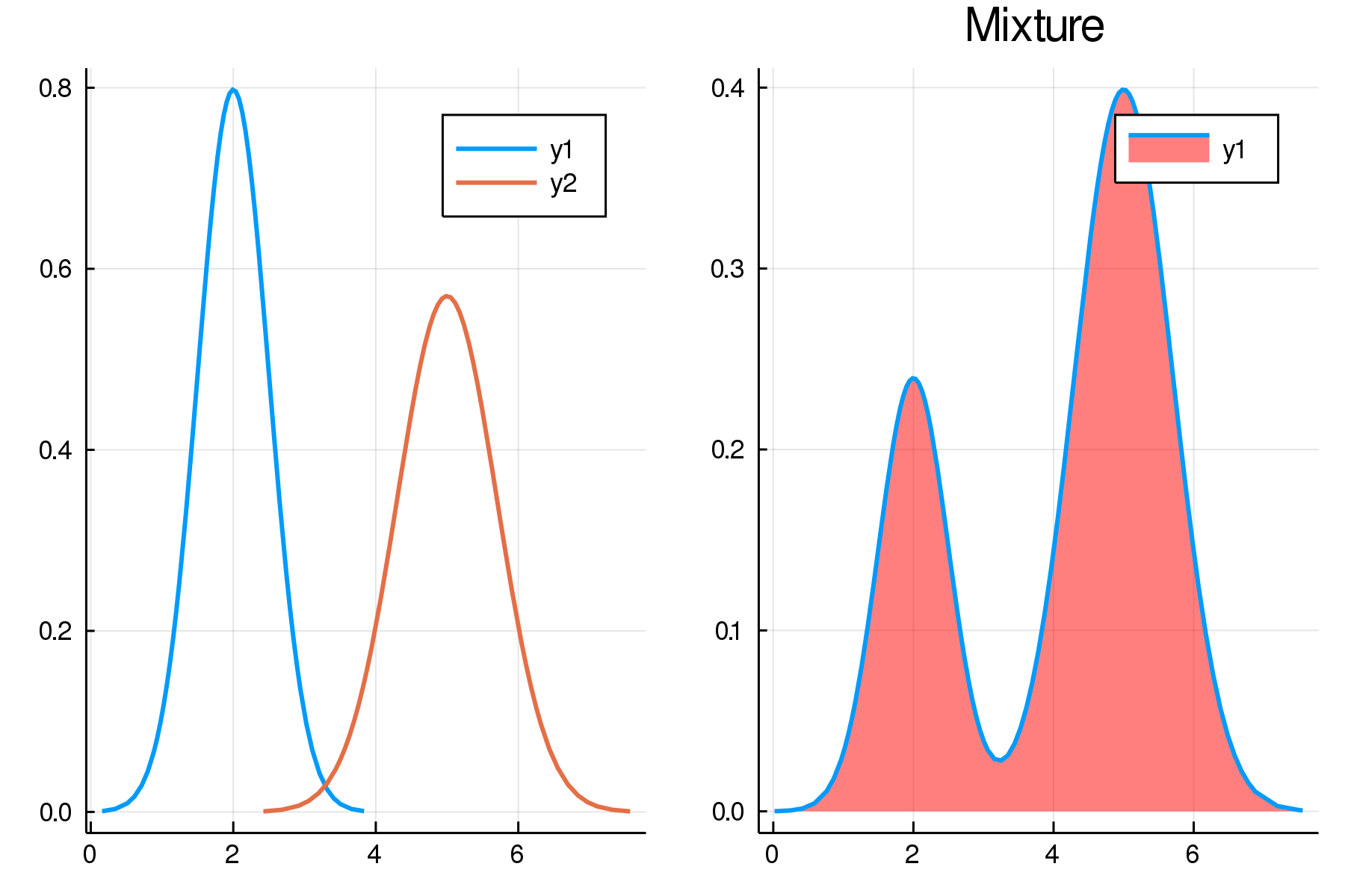
    if doplot
        plot(
            plot(m,linewidth=2), 
            plot(m,linewidth=2, fill=(0,:red,0.5), components = false, title="Mixture"),dpi = 300
            )
        savefig("mixtures.png")
    end
    y = rand(m,n)

    return Dict(:y => y, :μ => μ, :σ => σ, :α => α)
end

sets true mixture parameters
creates a Distributions.MixtureModel data type
optionally makes a plot from it
draws n random realizations from it

The setup looks like this:

All benchmarks will now proceed in the same way:

Take vector y
set (the same) wrong starting values
run the EM algorithm for iters iterations to find true values of proportion weights $\alpha$, means $\mu$ and variances $\sigma$ for each component.
Notice that the starting values are such that the algorithm never fully recovers the true values. Given it’s the same data, however, each implementation will follow the same path for parameter values and run the same number of iterations (again, none until convergence).

`julia` by hand

Here is my relatively naive and just-copy-thy-math implemenation in julia:

function bm_jl(y::Vector{Float64};iters=100)

    # poor starting values
    μ = [4.0,6.0]
    σ = [1.0,1.0]
    α = [0.5,0.5]

    N = length(y)
    K = length(μ)

    # initialize objects    
    L = zeros(N,K)
    p = similar(L)

    for it in 1:iters

        dists = [Normal(μ[ik], σ[ik] ) for ik in 1:K]

        # evaluate likelihood for each type 
        for i in 1:N
            for k in 1:K
                # Distributions.jl logpdf()
                L[i,k] = log(α[k]) + logpdf.(dists[k], y[i]) 
            end
        end

        # get posterior of each type 
        p[:,:] = exp.(L .- logsumexp(L))
      
        # with p in hand, update 
        α[:] .= vec(sum(p,dims=1) ./ N)
        μ[:] .= vec(sum(p .* y, dims = 1) ./ sum(p, dims = 1))
        σ[:] .= vec(sqrt.(sum(p .* (y .- μ').^2, dims = 1) ./ sum(p, dims = 1)))
    end
    return Dict(:α => α, :μ => μ, :σ => σ)
end

`GaussianMixtures.jl`

Next is a julia package written for this purpose. Here is the relevant part:

function bm_jl_GMM(y::Vector{Float64};iters=100)
    gmm = GMM(2,1)  # initialize an empty GMM object
    # stick in our starting values
    gmm.μ[:,1] .= [4.0;6.0]
    gmm.Σ[:,1] .= [1.0;1.0]
    gmm.w[:,1] .= [0.5;0.5]

    # run em!
    em!(gmm,y[:,:],nIter = iters)
    return gmm
end

`R` not-so-naive by hand

I tried to vectorize as much as possible here
Self-imposed rules: no Rcpp
You can see this uses an R-string, where data values are interpolated with a $ into the R session.

# this is a julia function!
function bm_R(y;iters=100)
    
    # that defines an R-string, sent off to R.
    r_result = R"""

    library(tictoc)

    # define a `repeat` function
    spread <- function (A, loc, dims) {
        if (!(is.array(A))) {
            A = array(A, dim = c(length(A)))
        }
        adims = dim(A)
        l = length(loc)
        if (max(loc) > length(dim(A)) + l) {
            stop("incorrect dimensions in spread")
        }
        sdim = c(dim(A), dims)
        edim = c()
        oi = 1
        ni = length(dim(A)) + 1
        for (i in c(1:(length(dim(A)) + l))) {
            if (i %in% loc) {
                edim = c(edim, ni)
                ni = ni + 1
            }
            else {
                edim = c(edim, oi)
                oi = oi + 1
            }
        }
        return(aperm(array(A, dim = sdim), edim))
    }

    # define row-wise logsumexp
    logRowSumExp <- function(M) {
        if (is.null(dim(M))) {return(M)}
        vms = apply(M,1,max)
        log(rowSums(exp(M-spread(vms,2,dim(M)[2])))) + vms
    }

    # define the function to be timed in R
    simpleEM <- function(y,iters){
    
        K = 2
        N = length($y)
        
        EMfun <- function(mu,sigma,alpha,iters){
            # allocate arrays
            p = array(0,c(N,K))
            L = array(0,c(N,K))
            
            for (it in 1:iters){
                # E step
                
                # vectorized over N loop
                for (k in 1:K){
                    L[ ,k] = log(alpha[k]) + dnorm(y,mean = mu[k], sd = sigma[k], log = TRUE)
                }
                p = exp(L - logRowSumExp(L))
                
                # M step
                alpha = colMeans(p)
                mu = colSums(p * y) / colSums(p)
                sigma = sqrt( colSums( p * (y - spread(mu,1,N))^2 ) / colSums(p) )
            }
            o =list(alpha=alpha,mu=mu,sigma=sigma)
            return(o)
        }
        
        # starting values
        mu_    = c(4.0,6.0)
        sigma_ = c(1.0,1.0)
        alpha_ = c(0.5,0.5)

        # take time
        tic()
        out = EMfun(mu_,sigma_,alpha_,iters)
        tt = toc()
        return(list(result = out, time = tt$toc - tt$tic))
    }
    simpleEM($y,$iters)   # run function in R!
    """
    return r_result
end

`R mixtools` package

The mixtools package is a very mature and highly optimized package for EM estimation. Most of the computationally intensive parts are written in C^[For example, in the package source, look for src/normpost.c which evaluates the matrix of posterior probabilities, object p in the julia code above. ]. My call:

function bm_R_mixtools(y::Vector{Float64};iters=100)
    
    r_result = R"""

    library(tictoc)
    library(mixtools)

    mu    = c(4.0,6.0)
    sigma = c(1.0,1.0)
    alpha = c(0.5,0.5)

    y = $y
    N = length(y)
    K = 2
    iters = $iters
    
    tic()
    result = normalmixEM(y,k = K,lambda = alpha, mu = mu, sigma = sigma, maxit = iters)
    tt = toc()
    list(result = result, time = tt$toc - tt$tic)

    """
    return r_result
end

Results!

I use the BenchmarkTools.jl package to benchmark the julia functions. This runs the functions multiple times to account for system noise. (running multiple times also gets rid of any JIT-related delays in julia)
The R functions are timed within the R process using the tictoc package, so even if there were any significant overhead from RCall.jl, the measurement is immune to that.

Here is the output table, with n for sample size, and times in seconds:

n	jl	jlg	R	Rmix
10000	0.0388268	0.0179957	0.457	0.073
100000	0.366047	0.16506	5.068	0.889
1000000	3.99279	1.75384	47.522	8.344
10000000	46.833	31.4021	553.783	65.379

And a much clearer picture using log scales:

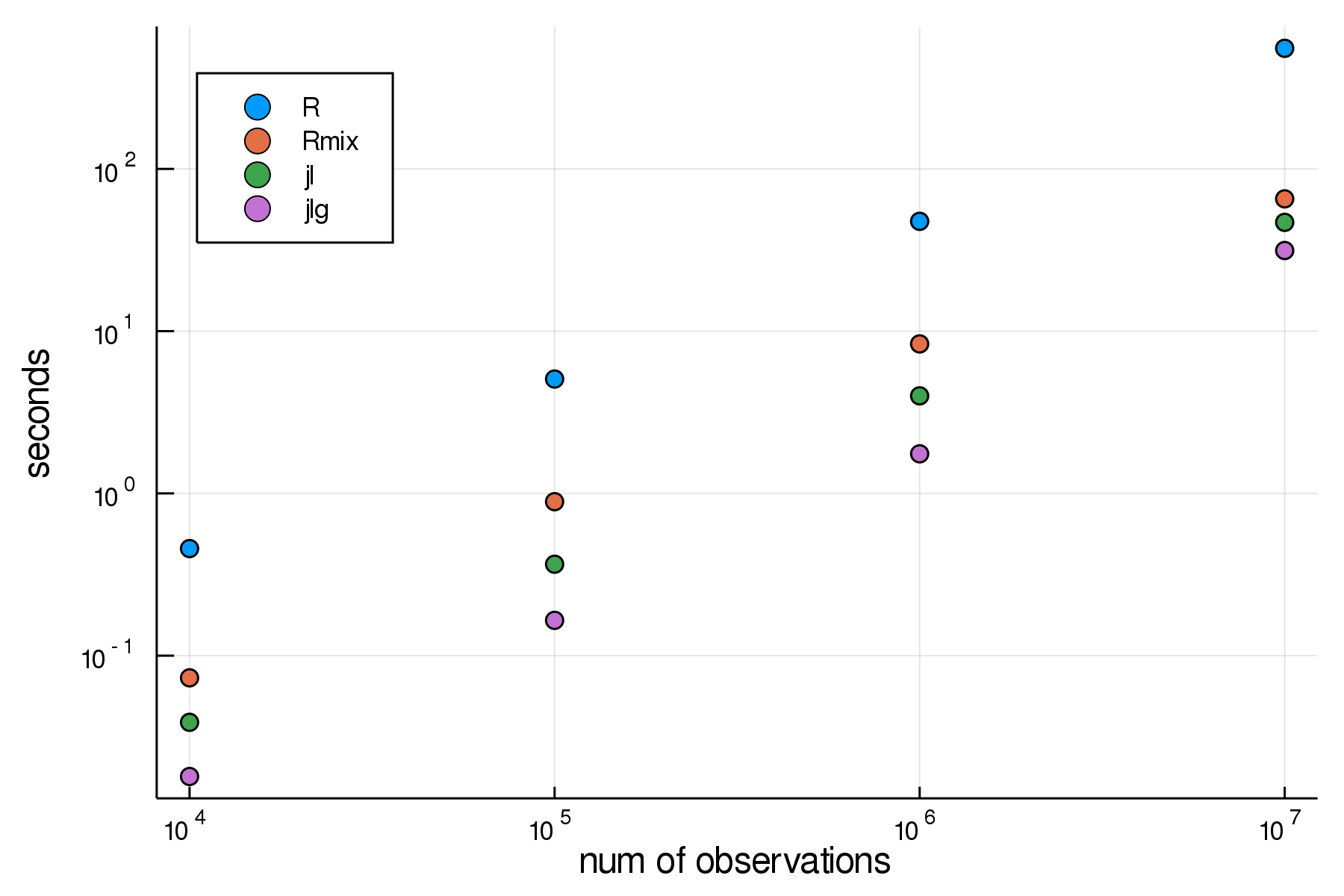
Conclusions

The naively hand-written code in julia performs very well.
The GaussianMixtures.jl performs best throughout
Both julia implementations outperform the C-optimized R mixtools package.
The vectorized R version comes in slowest.

I take from this that focusing on extending the work in GaussianMixtures.jl for my purposes is the most promising avenue here.

Code and Versions

Code is on github with full package version manifest.

julia> versioninfo()
Julia Version 1.1.0
Commit 80516ca202 (2019-01-21 21:24 UTC)
Platform Info:
  OS: macOS (x86_64-apple-darwin14.5.0)
  CPU: Intel(R) Core(TM) i5-5257U CPU @ 2.70GHz
  WORD_SIZE: 64
  LIBM: libopenlibm
  LLVM: libLLVM-6.0.1 (ORCJIT, broadwell)

shell> R --version
R version 3.5.1 (2018-07-02) -- "Feather Spray"
Copyright (C) 2018 The R Foundation for Statistical Computing
Platform: x86_64-apple-darwin15.6.0 (64-bit)

R is free software and comes with ABSOLUTELY NO WARRANTY.
You are welcome to redistribute it under the terms of the
GNU General Public License versions 2 or 3.
For more information about these matters see
http://www.gnu.org/licenses/.

R julia computing

EM Benchmarks

Weapon of Choice?

Benchmark Setup

`julia` by hand

`GaussianMixtures.jl`

`R` not-so-naive by hand

`R mixtools` package

Results!

Conclusions

Code and Versions

Florian Oswald

Associate Professor of Economics

EM Benchmarks

Weapon of Choice?

Benchmark Setup

julia by hand

GaussianMixtures.jl

R not-so-naive by hand

R mixtools package

Results!

Conclusions

Code and Versions

Florian Oswald

Associate Professor of Economics

`julia` by hand

`GaussianMixtures.jl`

`R` not-so-naive by hand

`R mixtools` package